0. To do list

hPES 논문읽기

논문 읽기

MNIST 분류

해보자해보자

layer 쌓기쌓기

backpropagation 잘 생각해봐서 해보면 좋을듯함.

논문 읽어서 idea 얻기

논문들
SNN에서 backpropagation 쓴것
https://www.readcube.com/articles/10.3389/fnins.2016.00508
https://s3-us-west-2.amazonaws.com/secure.notion-static.com/a866e23a-c395-493d-8c2e-2e48a6bdf194/Lee_et_al-2016-Frontiers_in_Neuroscience.pdf
https://s3-us-west-2.amazonaws.com/secure.notion-static.com/c06005dd-98c4-4da5-a384-20e6c3a09086/fnins-14-00119.pdf

Eliasmith 교수님 논문. tuning curve를 activation function으로 사용하고 미분 가능한 soft LIF를 사용하여 DNN 으로 구현.
https://s3-us-west-2.amazonaws.com/secure.notion-static.com/bc42a6fe-d08d-4367-9b3a-c064029a97cd/1510.08829.pdf

NEF - nengo 공부

nengo 홈페이지에서 python 으로 작성된 NEF 공부. (현우님이 알려주신거)

1. hPES

Simultaneous unsupervised and supervised learning of cognitive functions in biologically plausible spiking neural networks

https://s3-us-west-2.amazonaws.com/secure.notion-static.com/7aea94c3-f58c-4ff3-98ab-2fdf174016b0/qt9k64b389_noSplash_bccc8b60960ad5b93390f23ad99056df.pdf

What is the semantic pointers?
Semantic pointers are symbol-like representations that result from the compression and recursive binding of perceptual, lexical, and motor representations, effectively integrating traditional connectionist and symbolic approaches.

같은 저자라서 method 내용들이 저번에 정리한 NEF부분과 상당히 겹처서 나름 읽기 수월하였음. (이전에 읽었을때는 주요 포인트만 읽고 대부분 훑기만 하였음)

hPES (homeostatic Prescribed Error Sensitivity) rule

homeostasis 항상성 이란 뜻을 가지고 있음.

spiking BCM + PES rule

BCM 으로 sparsification

PES 로 supervised learning.

$\Delta w_{ij} = \kappa \alpha_j a_i(S \bold e_j \cdot \bold E + (1-S)a_j(a_j-\theta))$

$0 \leq S \leq 1$ 이기 때문에 PES term 과 BCM term 이 적절히 섞여 있는 형태.

hPES

STDP rule 과 동등함.

BCM term으로 인하여 frequency dependence 있음 (=triplet STDP)

weight matrix 가 sparse 해짐.

→ BCM term 때문. 단순 BCM 이면 sparse 해지는 대신, accuracy 감소. but hPES는 PES term 때문에 감소 x.

sparsity of weight matrix 가 높으면 왜 좋은거지?

대충 생각해봤을때는 Dropout 처럼 되서 overfitting 덜된다 (random이 아니라 fixed 이므로 이건 아닐듯.) or energy, 메모리 감소.

hPES 인지기능 가능.

당시 MNIST 가 고차원 정보였나 봄. high dimensional spaces 에도 적용 가능하다고 하면서 MNIST 로 기존 모델 (Spaun, PES) 보다 accuracy 가 높아진걸 보여줌.

PES learning 만으로 MNIST 96.31%

method에서 MNIST (28*28) → 50 차원의 semantic pointer 로 압축했다고 나와있음. (deep belif net 이용) 우리와 상황이 약간 다름.

2. MNIST classification

gpu 쓰는 code

with nengo_dl.Simulator(model,device='/gpu:0') as sim:

    sim.run(650)

Colab 기준 속도차이

nengo simulator 종류	30s 걸린시간	650s 걸린시간
nengo	8:25 (8:11)	?
nengo_dl (cpu)	2:04 (1:42)	7:45
nengo_dl (gpu)	2:55 (2:37)	28:24
nengo_ocl	1:12 (0:56)	19:48
nengo_mpi, nengo_spinnaker	설치가 안되거나 실행이 안됌.	설치가 안되거나 실행이 안됌.

stop_learning (inhibition) 하는 부분의 transform에서-20 을 쓰는 이유는?!

accuracy 할때 range로 뛰엄뛰엄 test 해야함

650s (1000장 500s train, 300장 150s test)

train acc: 0.983 test acc: 0.5666666666666667

train acc: 0.9945 test acc: 0.705

_ocl 이 보통 더 적은데 특별한 이유가 있는건지 아니면 우연히 그런건지...

Idea

population activity 가 이전 data에 영향을 받아서 높은 label이 떨어지는데 좀걸림. reset 같이 또는 쉬는 타임 을 넣어보면...?! tuning curve 가 음수쪽도 있어서 neuorn ensemble 을 inhibit 해서 해야할듯함. 나중에 해보자.

데이터를 아까 hPES 처럼 차원축소 해서 넣어주면 더 좋을거 같은데 따로 처리해서 넣는건 굳이 SNN 쓸 필요가 없으니 SNN형태로. 이전에 공부할때 hebbian learning 이 PCA 한다고 하니 이를 이용해서 어떻게 하면...?!
https://s3-us-west-2.amazonaws.com/secure.notion-static.com/eddd46a6-274c-4153-ac32-0b79f6fb66c2/7.1_Synaptic_Plasticity_Hebbs_Rule_and_Statistical_Learning.pdf

시간이 없어서 구현은 좀...

3. layer 쌓기 쌓기

미루면 안되는데... 미뤄야... ㅜ.ㅜ

논문들 읽고 생각정리해서 해볼예정...(시간이 된다면...)

논문들
SNN에서 backpropagation 쓴것
https://www.readcube.com/articles/10.3389/fnins.2016.00508
https://s3-us-west-2.amazonaws.com/secure.notion-static.com/a866e23a-c395-493d-8c2e-2e48a6bdf194/Lee_et_al-2016-Frontiers_in_Neuroscience.pdf
https://s3-us-west-2.amazonaws.com/secure.notion-static.com/c06005dd-98c4-4da5-a384-20e6c3a09086/fnins-14-00119.pdf

Eliasmith 교수님 논문. tuning curve를 activation function으로 사용하고 미분 가능한 soft LIF를 사용하여 DNN 으로 구현.
https://s3-us-west-2.amazonaws.com/secure.notion-static.com/bc42a6fe-d08d-4367-9b3a-c064029a97cd/1510.08829.pdf

4. NEF

nengo 에서 NEF를 python으로 구현해놓은거 (현우님이 알려주신거)

The NEF algorithm - Nengo 3.2.0.dev0 docs

While Nengo provides a flexible, general-purpose approach to neural modelling, some aspects rely on the Neural Engineering Framework (NEF) to help specify network behavior. The theory behind the Neural Engineering Framework is developed at length in Eliasmith & Anderson, 2003: "Neural Engineering" and a short summary is available in Stewart, 2012: "A Technical Overview of the Neural Engineering Framework".

https://www.nengo.ai/nengo/examples/advanced/nef-algorithm.html

일단 이전에 NEF는 temporal coding 과 rate coding 사이라고 정리했었는데, 그 이유는 single neuron model에서 spike가 나타나게 되고 이를 통해서 rate coding 처럼 여러 neuron에 걸쳐서 얻게 되기 때문이다. 정확히는 population coding 이다. 사실 정리하면서 조금 애매하게 아는거 같아서 이 code를 보고 확실히 넘어가자. (NEF를 공부 했지만 nengo 구현이랑 완벽하게 이어지지 않아서 보기로 결정!)

1. Introduction

%matplotlib inline

import math
import random

import numpy
import matplotlib.pyplot as plt

dt = 0.001  # simulation time step
t_rc = 0.02  # membrane RC time constant
t_ref = 0.002  # refractory period
t_pstc = 0.1  # post-synaptic time constant
N_A = 50  # number of neurons in first population
N_B = 40  # number of neurons in second population
N_samples = 100  # number of sample points to use when finding decoders
rate_A = 25, 75  # range of maximum firing rates for population A
rate_B = 50, 100  # range of maximum firing rates for population B


def input(t):
    """The input to the system over time"""
    return math.sin(t)


def function(x):
    """The function to compute between A and B."""
    return x * x

LIF neuron으로 simple feed forward 구현. 각 connection은 특정 함수를 계산 하도록 최적화됌. (NEF에서 decoding)

A,B 각각 50개,40개의 neuron population으로 구현을 할 예정이고, input은 sin wave, A→B 연결은 $x^2$ 이 되도록 하겠다.

(나머지 상수들은 설명 생략)

N_samples 는 무엇인지 나중에 체크

2. Initialization

A,B population에서 encoding vector 를 뉴런수 만큼 구현.

1D 라서 1,-1 2개의 값만 가짐.

# create random encoders for the two populations
encoder_A = [random.choice([-1, 1]) for i in range(N_A)]
encoder_B = [random.choice([-1, 1]) for i in range(N_B)]

#ex) [1,1,-1,1,-1, ...,-1]

gain과 bias 를 구함.

intercept는 firing 하기 시작하는 x value인데 threshold 같은 느낌인듯.

z는 0~inf 값을 갖고 수식적으로 $J \over J^{th}$ 값이라서 input (J) 비례함.

g 는 gain, b 는 bias 인데 왜이렇게 정의하는지 좀더 생각해봐야함.

gain은 alpha, bias 는 J_bias 일텐데 본디 이 값은 neuron의 intrinsic 한 value

def generate_gain_and_bias(count, intercept_low, intercept_high, rate_low, rate_high):
    gain = []
    bias = []
    for _ in range(count):
        # desired intercept (x value for which the neuron starts firing
        intercept = random.uniform(intercept_low, intercept_high)
        # desired maximum rate (firing rate when x is maximum)
        rate = random.uniform(rate_low, rate_high)

        # this algorithm is specific to LIF neurons, but should
        # generate gain and bias values to produce the desired
        # intercept and rate
        z = 1.0 / (1 - math.exp((t_ref - (1.0 / rate)) / t_rc))
        g = (1 - z) / (intercept - 1.0)
        b = 1 - g * intercept
        gain.append(g)
        bias.append(b)
    return gain, bias


# random gain and bias for the two populations
gain_A, bias_A = generate_gain_and_bias(N_A, -1, 1, rate_A[0], rate_A[1])
gain_B, bias_B = generate_gain_and_bias(N_B, -1, 1, rate_B[0], rate_B[1])

neuron model

( $\tau_{rc} {dV \over dt} = -V + IR$ ) LIF 기본식 + refractory period, spike (threshold) 정의.

각 neuron voltage 를 dt만큼 지났을때 spike list retrun

def run_neurons(input, v, ref):
    """Run the neuron model.

    A simple leaky integrate-and-fire model, scaled so that v=0 is resting
    voltage and v=1 is the firing threshold.
    """
    spikes = []
    for i, _ in enumerate(v):
        dV = dt * (input[i] - v[i]) / t_rc  # the LIF voltage change equation
        v[i] += dV
        if v[i] < 0:
            v[i] = 0  # don't allow voltage to go below 0

        if ref[i] > 0:  # if we are in our refractory period
            v[i] = 0  # keep voltage at zero and
            ref[i] -= dt  # decrease the refractory period

        if v[i] > 1:  # if we have hit threshold
            spikes.append(True)  # spike
            v[i] = 0  # reset the voltage
            ref[i] = t_ref  # and set the refractory period
        else:
            spikes.append(False)
    return spikes

input J 계산 ( $J = \alpha \bold e \cdot \bold x + J^{bias}$ )

t가 time_limit 될때까지 run_neuron 함수에서 spike 계산하고 spike rate return

def compute_response(x, encoder, gain, bias, time_limit=0.5):
    """Measure the spike rate of a population for a given value x."""
    N = len(encoder)  # number of neurons
    v = [0] * N  # voltage [0,0,...,0]
    ref = [0] * N  # refractory period

    # compute input corresponding to x
    input = []
    for i in range(N):
        input.append(x * encoder[i] * gain[i] + bias[i])
        v[i] = random.uniform(0, 1)  # randomize the initial voltage level

    count = [0] * N  # spike count for each neuron

    # feed the input into the population for a given amount of time
    t = 0
    while t < time_limit:
        spikes = run_neurons(input, v, ref)
        for i, s in enumerate(spikes):
            if s:
                count[i] += 1
        t += dt
    return [c / time_limit for c in count]  # return the spike rate (in Hz)

tuning curve 계산.

x_values [-1, -0.98,...,1]

input x 에 따른 spike rate 계산 → A

def compute_tuning_curves(encoder, gain, bias):
    """Compute the tuning curves for a population"""
    # generate a set of x values to sample at
    x_values = [i * 2.0 / N_samples - 1.0 for i in range(N_samples)]

    # build up a matrix of neural responses to each input (i.e. tuning curves)
    A = []
    for x in x_values:
        response = compute_response(x, encoder, gain, bias)
        A.append(response)
    return x_values, A

decoder vector $\bold d = (\bold A \bold A^T)^{-1} \bold A \bold X^T$ 구하는 이 식으로 계산.

def compute_decoder(encoder, gain, bias, function=lambda x: x):
    # get the tuning curves
    x_values, A = compute_tuning_curves(encoder, gain, bias)

    # get the desired decoded value for each sample point
    value = numpy.array([[function(x)] for x in x_values])

    # find the optimal linear decoder
    A = numpy.array(A).T
    Gamma = numpy.dot(A, A.T)
    Upsilon = numpy.dot(A, value)
    Ginv = numpy.linalg.pinv(Gamma)
    decoder = numpy.dot(Ginv, Upsilon) / dt
    return decoder

decoder A, B계산.

weight matrix 가 왜 이렇게 되는지 생각해봐야할듯.

weight component 가 $w_{ij} = \alpha_j \bold e_j \cdot \bold d_i$ 이렇게 되어서 그런듯한데 gain도 곱해야 하지 않나.

# find the decoders for A and B
decoder_A = compute_decoder(encoder_A, gain_A, bias_A, function=function)
decoder_B = compute_decoder(encoder_B, gain_B, bias_B)

# compute the weight matrix
weights = numpy.dot(decoder_A, [encoder_B]

3. Running the simulation

post-synaptic filter $h(t) = {1 \over \tau^{pstc}} e^{-{t \over \tau^{pstc}}}$ 이므로

input 으로 받는경우

pstc_scale = $1-h'(dt) = 1-e^{-{t \over \tau^{pstc}}}$ 만큼 곱해진다고 생각해도됌

leakage 는 1-pstc_scale 곱해진다고 생각 가능.

A → B running

(encoder,decoder 는 이미 정해졌고 simulation 되면서 input,spike,output 이 바뀜.)

v_A = [0.0] * N_A  # voltage for population A
ref_A = [0.0] * N_A  # refractory period for population A
input_A = [0.0] * N_A  # input for population A

v_B = [0.0] * N_B  # voltage for population B
ref_B = [0.0] * N_B  # refractory period for population B
input_B = [0.0] * N_B  # input for population B

# scaling factor for the post-synaptic filter
pstc_scale = 1.0 - math.exp(-dt / t_pstc)

# for storing simulation data to plot afterward
inputs = []
times = []
outputs = []
ideal = []

output = 0.0  # the decoded output value from population B
t = 0
while t < 10.0:  # noqa: C901 (tell static checker to ignore complexity)
    # call the input function to determine the input value
    x = input(t)

    # convert the input value into an input for each neuron
    for i in range(N_A):
        input_A[i] = x * encoder_A[i] * gain_A[i] + bias_A[i]

    # run population A and determine which neurons spike
    spikes_A = run_neurons(input_A, v_A, ref_A)

    # decay all of the inputs (implementing the post-synaptic filter)
    for j in range(N_B):
        input_B[j] *= 1.0 - pstc_scale
    # for each neuron that spikes, increase the input current
    # of all the neurons it is connected to by the synaptic
    # connection weight
    for i, s in enumerate(spikes_A):
        if s:
            for j in range(N_B):
                input_B[j] += weights[i][j] * pstc_scale

    # compute the total input into each neuron in population B
    # (taking into account gain and bias)
    total_B = [0] * N_B
    for j in range(N_B):
        total_B[j] = gain_B[j] * input_B[j] + bias_B[j]

    # run population B and determine which neurons spike
    spikes_B = run_neurons(total_B, v_B, ref_B)

    # for each neuron in B that spikes, update our decoded value
    # (also applying the same post-synaptic filter)
    output *= 1.0 - pstc_scale
    for j, s in enumerate(spikes_B):
        if s:
            output += decoder_B[j][0] * pstc_scale

    if t % 0.5 <= dt:
        print(t, output)
    times.append(t)
    inputs.append(x)
    outputs.append(output)
    ideal.append(function(x))
    t += dt

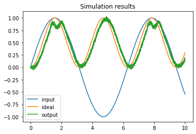
4. Plot the results

x, A = compute_tuning_curves(encoder_A, gain_A, bias_A)
x, B = compute_tuning_curves(encoder_B, gain_B, bias_B)

plt.figure()
plt.plot(x, A)
plt.title("Tuning curves for population A")

plt.figure()
plt.plot(x, B)
plt.title("Tuning curves for population B")

plt.figure()
plt.plot(times, inputs, label="input")
plt.plot(times, ideal, label="ideal")
plt.plot(times, outputs, label="output")
plt.title("Simulation results")
plt.legend()
plt.show()

Tuning curve 에서

encoder 통해서 -,+ 정해지고

intercept 통해서 activation value? 정해지고

rate 통해서 기울기 or upper bound 정해진다는 느낌.

이를 통해 만들어진 여러 neuron 들로 NEF 로 구현.

Uploaded by N2T

'Nengo' 카테고리의 다른 글

nengo - 8주차 (0)	2022.06.14
nengo-6주차-2 (0)	2022.06.14
nengo-6주차 (0)	2022.06.14
nengo 5주차 (0)	2022.06.14
nengo 하고싶은 것 (0)	2022.06.14

Untitled

nengo 7주차

0. To do list

1. hPES

2. MNIST classification

Colab 기준 속도차이

3. layer 쌓기 쌓기

4. NEF

1. Introduction

2. Initialization

3. Running the simulation

4. Plot the results

'Nengo' 카테고리의 다른 글

티스토리툴바

nengo 7주차

0. To do list

1. hPES

2. MNIST classification

Colab 기준 속도차이

3. layer 쌓기 쌓기

4. NEF

1. Introduction

2. Initialization

3. Running the simulation

4. Plot the results

'Nengo' 카테고리의 다른 글

'Nengo' Related Articles

티스토리툴바