Nengo

nengo-6주차-2

건강검진진료 2022. 6. 14. 00:03

Introduction

PES learning 에서 layer 를 쌓기 위해, 그리고 궁금증 (neuron 이 많이 필요한 이유, 2layer 로 $y=x^2$ regression 되는 이유, 생물학적 타당성)을 해결하기 위해 여러 자료를 찾던 중,

아래 자료를 발견하였다.

https://s3-us-west-2.amazonaws.com/secure.notion-static.com/903d9f27-cd56-4039-9e4a-508a4b055f95/bekolay_master_thesis(2011).pdf

bekolay 님의 석사학위논문인데, 정리가 잘 되어 있고 내가 얻고자 하는 부분이 어느정도 나와있는거 같아서 공부해보았다. (참고로 bekolay 는 waterloo 대학에서 Eliasmith 교수의 지도를 받아 석사,박사 학위를 취득하였다. nengo 논문의 1저자 이자 교신저자)

논문의 제목은 Learning in large-scale spiking neural networks 이지만 주된 내용은 NEF기반 생물학적 타당한 spiking neural network 으로 machine learning 구현이다.

chapter 1 은 학위논문의 introduction, chapter 2 는 synaptic plasticity 를 설명한다. Hebbian learning(LTP, LTD, STDP)을 주로 설명한다.

chapter 3 는 Large-scale neural modeling 으로 single neuron model 과 이를 기반으로 large scale 로 가기위한 NEF를 소개한다.

chapter 4 는 Supervised learning 으로, 기존 backpropagation 과 함게 NEF를 이용한 supervised learning 에 대하여 설명한다. 여기서 PES learning 내용이 나오지만 이름이 붙기 전이라서 PES 단어 자체는 없다.

chapter 5 는 Reinforcement learning, chapter 6 는 unsupervised learning 으로 NEF를 이용하여 구현한다.

chapter 7 에선 discussion and conclusion 으로 학위 논문이 마무리 된다.

내가 원하는 부분은 chapter 3,4 에 있어서 chapter 3,4를 정리하도록 하겠다.

Main

Chapter 3 Large-scale neural modeling

3.1 Single-neuron models

여러 모델이 있지만 가장 유명한 2개 모델

a) Hodgkin-Huxley model

많은 파라미터 미분방적식 으로 기술됌. (보통 ion channel dynamics 식 3개와 current 식1 개)

생물학적 특성을 잘 묘사하지만, 1ms simulation 하는데 1000 computations 이상 필요.

4개의 미분방정식

b) Leaky integrate-and fire model

수학적으로 매우 심플한 모델. 계산에 용이함.

1ms simulation 하는데 10 computations 이하 필요.

(2개의 모델의 중간쯤인 izhikevich 도 있다)

계산 편의성때문에 Leaky integrate-and fire model (LIF model) 사용

3.1.1 Leaky integrate-and fire model

Leaky integrate-and fire model 은

lipid bilayer에 의한 capacitor (C), ion channel을 resistor (R), membrane voltage (V), Input current (J 또는 J_M), threshold voltage(V_th) 를 이용하여 modeling 한다.

수식 다음과 같다.

${dV \over dt} = -{1 \over RC} (V(t) - J(t)R)$

derivation (LIF)
$\begin{align} J_{M} &= J_{R}+J_{C}\\ &={V \over R} + C{dV \over dt}\\ {dV \over dt} &= -{1 \over RC}(V(t)-J(t)R) \end{align}$

단순 RC circuit과 다르게 LIF neuron은 두개의 nonlinearity 가 있다.

V가 V_th 되면, spike 가 나오고 ( $\delta(t-t_{n})$ ) ,V는 0으로 reset된다.

spike가 나오면 refractory period ( $\tau_{ref}$ ) 가 있어서 한동안 강제적으로 V=0 이 된다.

3.2 The Neural Engineering Framework

NEF는 single-neuron 을 large-scale network 로 확장하기 위한 principle 모음이다.

(The Neural Engineering Framework (NEF) is a set of principles that can be used to build large-scale networks of single-neuron models.)

NEF 네는 3가지 principle 이 존재한다.

Representation

Transformation

Dynamics

여기서는 1,2 내용만 필요해서 1,2만 다룬다.

3.2.1 Representation

NEF 가정)

뇌에서 정보를 받으면 spike pattern 으로 encoding 한다고 가정한다.

Information —~~(encoding)~~—> spike patterns of neurons

즉, In NEF

vector —~~encoding~~—> spikes —~~decoding~~—> vector

따라서 NEF 에서 정의하는 Encoding Decoding 을 알아보자.

Encoding

single neuron model에서 input current J를 받으면 non-linear function G를 통하여 output spike가 발생. 따라서 neuron의 activity a는

$a(J) = G[J]$ 이렇게 쓸 수 있음.

sensory neuron을 기준으로 생각하면 input current J를 다음과 같이 쓸수 있음.

$J(x) = \alpha(\bold e \cdot \bold x) + J^{bias}$

$\bold x$ : 외부신호 (위치에 index로 가지는 빛 세기 벡터)

$\bold e$ : encoder unit vector (예를 들어 밝은 빛을 인지하면 1 반대면 -1 이런식인데 벡터로 확장 or 원추세포 RGB selectivity로 생각해도 될듯)

$\alpha$ : scailing factor 인데 이 뉴런의 sensitivity 라고 생각하면 됌.

$J^{bias}$ : 외부자극 없이 받는 current. noise나 intrinsic 한 특성이라 보면 될듯.

Decoding

encoding과 반대 process. spiking pattern을 vector로 mapping해야함.

(2진법 → 10진법 예시)

Decoing 식은 다음과 같다.

$\bold{\hat x} = \sum_{i}^{n} \bold d_i a_i$

$\bold {\hat x}$ 는 decode 된 결과물 (encoding 된 vector 예측)

$\bold d_i$ 는 i-th neuron의 decoing vector 이고, $a_i$ 는 i-th neruon의 activity

activity 식은 아래와 같이 된다. (input 에 따른 spike frequency) : Tuning curve

a(x) = \begin{cases} {1 \over {\tau^{ref} - \tau^{RC} \ln \left(1- {J^{th} \over {\alpha x +J^{bias}}} \right)}} &, \text{if } \alpha x+J^{bias} > J^{th} \\ 0 &, \text{otherwise} \end{cases}

derivation
현우님께서 저번에 해주셨음. 추후 추가 예정...

Decoding matrix $\bold d$ (decoding vector concat) 구하는 방법.

$\bold d = \bold \Gamma^{-1} \bold \Upsilon$

least-square minimization 하면 됌. regression 하듯이 하면 됌.

derivation
column vector 꼴이 익숙해서 이렇게 matrix를 정의하면
$\bold X = \begin{bmatrix} x_0 \\ x_1 \\ \vdots \\ x_t \end{bmatrix} \,\,\,\,\,\, \bold A = \begin{bmatrix} \bold a(x_0) \\ \bold a(x_1) \\ \vdots \\ \bold a(x_t) \end{bmatrix} \,\,\,\,\,\, \bold a(x) = \begin{bmatrix} a_0x & a_1x & \dots & a_n x \end{bmatrix}$
$\bold {\hat X} = \bold A \bold d$ 이렇게 쓸 수 있다. 따라서 error $\bold E$ 를 정의하면
$\bold E = \bold X - \bold {\hat X} = \bold X - \bold A \bold d$ 이다.
loss function (cost function) $L$ 은
$\begin{align} L &= ||\bold E||^2 \\ & = \bold E^T \bold E \\ &=(\bold X^T - \bold d^T \bold A^T)(\bold X- \bold A \bold d) \\ &= \bold X^T \bold X - \bold X^T \bold A \bold d - \bold d^T \bold A^T \bold X + \bold d^T \bold A^T \bold A \bold d \end{align}$
따라서 $\bold d$ 로 미분하면
$\begin{align} {\partial L \over \partial \bold d} &= -\bold A^T \bold X - \bold A^T \bold X+ \bold A^T \bold A \bold d + \bold A^T \bold A \bold d \\ & = 2\bold A^T \bold A \bold d - 2\bold A^T \bold X \end{align}$
loss function 을 최소화 하는 상황 → ${\partial L \over \partial \bold d} = \bold 0$ (least square error라서 convex 하므로 global minimum)
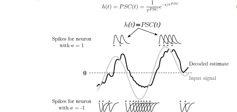
$\begin{align} 2\bold A^T \bold A \bold d - 2\bold A^T \bold X &= \bold 0 \\ \bold A^T \bold A \bold d &= \bold A^T \bold X \\ \bold d &= (\bold A^T \bold A)^{-1} \bold A^T \bold X \, \\ \text{thesis 처럼 column vector} &=> \text{row vector} \\ \bold d &= (\bold A \bold A^T)^{-1} \bold A \bold X^T \\ &= \bold \Gamma^{-1} \bold \Upsilon \\ \text{where }\, \bold \Gamma = \bold A \bold A^T \,\, &\text{and } \bold \Upsilon = \bold A \bold X^T \end{align}$

decoding 식에서 시간 term을 넣어보면 아래 수식처럼 쓸 수 있음.

\begin{align} \bold{\hat x} &= \sum_{i=0}^{n} \bold d_i a_i(t) \\ &= \sum_{i=0}^{n} \bold d_i \sum_{s} \delta (t-t_s) * h(t) \\ &= \sum_{i=0}^{n} \bold d_i \sum_{s} h(t-t_s) \\ \end{align}

$h(t)$ 는 filter 인데 아래 그림과 같이 PSC (post synaptic current)를 사용.

3.2.2 Transformation

대부분 neuron은 외부 환경에서 오는 input 보단 다른 neuron을 통해 input을 받음.

따라서 다른 neuron으로부터 온 input J

$J_j = \sum_{i=0}^n w_{ij}a_i + J_j^{bias}$

Linear transformation

$\bold y = \bold x$ —> simple transformation 해보자.

(x → encoding → ... → decoding → x )

second layer neuron 이 받는 current 식을 통해 w 를 구하면,

\begin{align} J_j &= \alpha_j (\bold e_j \cdot \bold x) + J_j^{bias}\\ &= \alpha_j (\bold e_j \cdot \sum_{i=0}^n \bold d_i a_i) + J_j^{bias}\\ &= \sum_{i=0}^n\alpha_j \bold e_j \cdot \bold d_i a_i + J_j^{bias}\\ \sum_{i=0}^n w_{ij}a_i + J_j^{bias}&= \sum_{i=0}^n\alpha_j \bold e_j \cdot \bold d_i a_i + J_j^{bias}\\ w_{ij} &= \alpha_j \bold e_j \cdot \bold d_i \end{align}

이렇게 된다.

만약 $\bold y = \bold C\bold x$ 일반적인 linear transformation case로 일반화 하면

$w_{ij} = \alpha_j \bold e_j \bold C_{ji} \bold d_i$ (i → j neuron synapse weight)

Nonlinear transformation

$f$ nonlinear function이 있을때 ( $\bold y = f(\bold x)$ case)

증명은 똑같음. 결론 식만 적으면

\bold d^{f(\bold x)} = \bold \Gamma^{-1} \bold \Upsilon \\ \text{where }\, \bold \Gamma = \bold A \bold A^T \,\, \text{and } \bold \Upsilon = \bold A f(\bold X^T)

$w_{ij} = \alpha_j \bold e_j \bold C_{ji} \bold d_i^{f(\bold x)}$ (i → j neuron synapse weight)

3.3 Plasticity in the NEF

w의 plasticity. learning rule에 따라 조정.

3.3.1 Error minimization rule

%% PES learning case. PES 이름 붙기전이라 단순히 least square 로 error minimization rule 이라고만 되어 있음.

least square error (SE)

\begin{align} SE &= - {1 \over 2}(\bold x - \bold {\hat x})^2 \\ &= - {1 \over 2}(\bold x - \sum_i \bold d_i a_i)^2 \\ {dSE \over d \bold d_i} &= (\sum_j \bold d_j a_j - \bold x)a_i\\ &= (\bold {\hat x} - \bold x)a_i\\ &= \bold Ea_i\\ \end{align}

따라서 $\Delta \bold d_i = \kappa \bold Ea_i$ 로 쓸 수 있다. ( $\kappa$ : learning rate , SE 는 -로 정의되어 커질수록 error가 적은거라 update 는 + 방향으로 함)

\begin{align} w_{ij} &= \alpha_j \bold e_j \cdot \bold d_i \text{ 이므로}\\ \Delta w_{ij} &= \alpha_j \bold e_j \cdot \Delta \bold d_i \\ &= \kappa \alpha_j \bold e_j \cdot \bold Ea_i \\ \end{align}

biological plausible 하지 않지만 backpropagation과 비교하면 locality 측면에서 좀더 plausible 함.

Chapter 4 Supervised learning

Supervised learning 이란 X, Y 가 주어질때 G(X) 를 추론하는것.

$\bold X -G(\bold X)-> \bold Y$

SNN 에서 supervised learning 문제

error signal 을 계산하는게 non trivial.

(label 은? 있다고 하더라도 spike 로 어떻게계산할지)

error signal 이 어떻게 connection weight 조절 할지.

(learning rule 문제)

4.1 Supervised learning in traditional artificial neural networks

machine learning 에서는 첫번째 문제는 문제아님. 두번째 문제는 backpropagation 알고리즘으로 해결가능.

Universal approximation theorem 의하여 3-layer(input-hidden-output) 로 모든 함수 근사 가능.

4.1.1 Backpropagation

a(x) 는 activation function ( snn 에선 tuning curve)

i → j connection weight 에서 learning rule 식은 다음과 같다.

$\Delta w_{ij} = -\kappa \delta_j a_i$

$\delta_j$ 는 neuron_j 의 local error

derivation
추후 작성 예정

SNN 에서는 activation function 은 spike를 generating 시키기 때문에 비연속적 및 미분 불가능. (기존 temporal coding)

게다가 backpropagation 은 biological plausible 하지 않음.

4.2 Supervised learning in spiking neural networks

실험적으로도 어떻게 supervised learning 하는지 데이터가 거의 없음. 그런데 cerebellar 연구에서 climbing fiber 에서 error signal 을 관측한 자료가 있음. 그렇지만 아직 supervised learning solution을 명확히 제공하지 않음.

While we have not found biologically plausible solutions to the general supervised learning problem, temporal-coding based solutions to the supervised spike-time learning problem exist.

4.2.1 Temporal-coding based models

temporal coding 기반 알고리즘 중 2개 소개.

SpikeProp 알고리즘 (2002)

backpropagation과 유사. global error 계산하고 정답 spike train 과 output spike train 의 시간차이를 local error 로하여 connection weight update함. (정확히는 first spike time coding)

local error가 뒷단 neuron weight에 의존하므로 생물학적 implausible.

이후 QuickProp, RProp 으로 발전됌. (time constant 나 threshold 추가)

ReSuMe (Remote supervised Method)

STDP 기반 알고리즘.

\Delta w_{ij} = - \Delta w_{ij}^{STDP} + \Delta w_{ik}^{STDP} \, \text{ for excitatory synpases} \\ \Delta w_{ij} = \Delta w_{ij}^{STDP} - \Delta w_{ik}^{STDP} \, \text{ for inhibitory synpases}\\

STDP rule 인데, teacher neruon 이 같이 개입된 형태. 실험적으로 관측된 STDP를 이용하지만, teacher neuron이 개입된 상태에서 update 해서 이 부분이 biological plausible 한지 불분명함.

4.2.2 Biologically plausible backpropagation

새로운 학습법보단 backpropagation 을 biological plausible 하게 만드는 접근 방법들 소개.

FreqProp

hebbian learning rule 에서 upgrade 된 느낌.

$\Delta w_{ij} = {1 \over N} \delta a_i a_j$ 형태. ( $\delta$ 는 output layer activity)

LEABRA (local error-driven associative biologically realistic algorithm)

등등이 있다.

4.3 Supervised learning with the NEF

이제 supervised learning 에서 생겼던 문제를 NEF 로 해결해보자.

((NEF 는 temporal coding 과 rate coding 중간이다.)

The NEF's coding scheme considers a small time window of spiking behaviour, making it somewhere in-between traditional rate coding and temporal coding schemes.

4.3.1 Theoretical argument

기존 문제는 2가지 이다.

1 error signal 계산 (biological plausible 하게)

2 weight update 어떻게? (biological plausible 하게)

NEF error-minimization (PES learning 이름 붙기전)

$\Delta w_{ij}= \kappa \alpha_j \bold e_j \cdot \bold Ea_i$ 이므로

2번문제는 해결가능.

1번 문제. Error 는 Error population 에서 계산되고, connection weight matrix 가 analytic 하게 결정되더라도 simple linear transformation이라 생물학적으로 불가능 하지 않음.

backpropagation 과 비교해보면

$\delta_j$ 는 neuron_j 의 local error.

backpropagation 동작과 같지만, error space 에서 어디가 sensitivity 한지 prescribe 해주기 때문에 backpropagation (downstram neuron 으로부터 backward propagation)을 요구하지 않음.

단점으로 bacpropagation 보다 hidden layer 에서 덜 flexible 해서 (?느낌은 오는데 정확히는 잘 모르겠음) 기존 NN 보다 더 많은 뉴런이 필요함. biological plausible 생각하면 작은비용이라고 주장함.

추가)

NEF에서 input - output 에서도 3 layer 로 봐야함. input 들어갈때 nonlinear process 가 있기 때문. 따라서 Universal Approximation Theorem 에 의하여 임의함수 가능함.

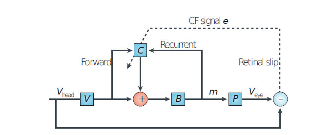
4.3.2 Biological plausibility

위 network 가 진짜 biological plausible 하는지 논의.

cerebellum 에서 비슷한 network 형태 가 존재

learning rule 이 local 하고, synapse 에 적용가능.

각 parameter 를 살펴보면

$\kappa$ : learning rate. biophysical model 에서 여러 scalar factor 합쳐진거라고 생각 가능.

$\alpha_j$ : gain factor. intrinsic 한 neuron property 로 생각 가능

$a_i$ : presynaptic cell의 activity

$\bold E$ : modulatory signal projected to error

dopamine level 로 생각하거나 neural activity 흔적 (cerebellum) 으로 생각 가능.

$e_j$ : encoding vector

sensory neuron 일 경우 intrinsic property

다른 neuron 이라도 synapse 위치가 반영된 term 이라고 생각 가능. (synpase - dendrite 위치에 따라 영향받기 때문)

이러한 이유들로 biological plausible 함.

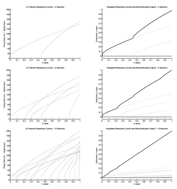
4.3.3 Simulation results, 4.3.4 Conclusion 내용은 생략하고 결과 그림아래.

My comment

<수정해야함>

with nengo_dl.Simulator(model,device='/gpu:0') as sim:
    sim.run(500)

—

정리를 위한 이미지

Uploaded by N2T