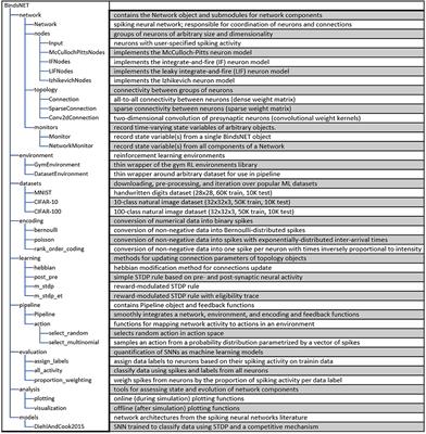
7주차 BindsNET tutorial
https://github.com/BindsNET/bindsnet
Part I: Creating and Adding Network Components
Creating a Network
from bindsnet.network import Network

network = Network()bindsnet.network.Networkobject
dt : time step (ms)
batch_size : minibatch size of the input data
learning : update to adaptave parameters of network component
reward_fn : reward signal
Adding Network Components
nodes : layers of neurons
bindsnet.network.topology : connections (Connection)
bindsnet.network.monitors : recording the state variables (Monitor)
Creating and adding layers
from bindsnet.network.nodes import LIFNodes

layer = LIFNodes(n=100, shape=(10,10))

# network.layer['LIF population'] <- access
network.add_layer(
		layer=layer, name="LIF population"
)bindsnet.network.nodesobject
n: the number of nodes in the layer
shape : the arrangement of the layer
thresh : threshold voltage
rest : resting voltage
trace : spike traces or not
tc_decay : time constant(voltage decay)
Etc... (Input, McCullochPitts, AdaptiveLIFNodes, IzhikevichNodes)
Creating and adding connections
from bindsnet.network.nodes import Input, LIFNodes
from bindsnet.network,topology import Connection

source_layer = Input(n=100)
target_layer = LIFNodes(n=1000)

# all-to-all connection
connection = Connection(
		source=source_layer, target=target_layer
)
Connection
source, target, w, b, wmin, wmax, update_rule
network.add_layer(
    layer=source_layer, name="A"
)
network.add_layer(
    layer=target_layer, name="B"
)
network.add_connection(
    connection=connection, source="A", target="B"
)add_connectionfunction
Specifying monitors
from bindsnet.network import Network
from bindsnet.network.nodes import Input, LIFNodes
from bindsnet.network.topology import Connection
from bindsnet.network.monitors import Monitor

network = Network()

source_layer = Input(n=100)
target_layer = LIFNodes(n=1000)

connection = Connection(
    source=source_layer, target=target_layer
)

# Create a monitor.
monitor = Monitor(
    obj=target_layer,
    state_vars=("s", "v"),  # Record spikes and voltages.
    time=500,  # Length of simulation (if known ahead of time).
)Monitorobject
network.add_layer(
    layer=source_layer, name="A"
)
network.add_layer(
    layer=target_layer, name="B"
)
network.add_connection(
    connection=connection, source="A", target="B"
)
network.add_monitor(monitor=monitor, name="B")add_monitorfunction
from bindsnet.network.monitors import NetworkMonitor

network_monitor = NetworkMonitor(
    network: Network,
    layers: Optional[Iterable[str]],
    connections: Optional[Iterable[Tuple[str, str]]],
    state_vars: Optional[Iterable[str]],
    time: Optional[int],
)
bindsnet.network.monitors.NetworkMonitor
Recording many network componets at once
Running Simulations
import torch
import matplotlib.pyplot as plt
from bindsnet.network import Network
from bindsnet.network.nodes import Input, LIFNodes
from bindsnet.network.topology import Connection
from bindsnet.network.monitors import Monitor
from bindsnet.analysis.plotting import plot_spikes, plot_voltages


# Simulation time.
time = 500

# Create the network.
network = Network()

# Create and add input, output layers.
source_layer = Input(n=100)
target_layer = LIFNodes(n=1000)

network.add_layer(
    layer=source_layer, name="A"
)
network.add_layer(
    layer=target_layer, name="B"
)

# Create connection between input and output layers.
forward_connection = Connection(
    source=source_layer,
    target=target_layer,
    w=0.05 + 0.1 * torch.randn(source_layer.n, target_layer.n),  # Normal(0.05, 0.01) weights.
)

network.add_connection(
    connection=forward_connection, source="A", target="B"
)

# Create recurrent connection in output layer.
recurrent_connection = Connection(
    source=target_layer,
    target=target_layer,
    w=0.025 * (torch.eye(target_layer.n) - 1), # Small, inhibitory "competitive" weights.
)

network.add_connection(
    connection=recurrent_connection, source="B", target="B"
)

# Create and add input and output layer monitors.
source_monitor = Monitor(
    obj=source_layer,
    state_vars=("s",),  # Record spikes and voltages.
    time=time,  # Length of simulation (if known ahead of time).
)
target_monitor = Monitor(
    obj=target_layer,
    state_vars=("s", "v"),  # Record spikes and voltages.
    time=time,  # Length of simulation (if known ahead of time).
)

network.add_monitor(monitor=source_monitor, name="A")
network.add_monitor(monitor=target_monitor, name="B")

# Create input spike data, where each spike is distributed according to Bernoulli(0.1).
input_data = torch.bernoulli(0.1 * torch.ones(time, source_layer.n)).byte()
inputs = {"A": input_data}

# Simulate network on input data.
network.run(inputs=inputs, time=time)

# Retrieve and plot simulation spike, voltage data from monitors.
spikes = {
    "A": source_monitor.get("s"), "B": target_monitor.get("s")
}
voltages = {"B": target_monitor.get("v")}

plt.ioff()
plot_spikes(spikes) #raster plot
plot_voltages(voltages, plot_type="line") # voltage
plt.ylim([-80,-50])
plt.show()

Simulation Notes
clock-driven simulation
Q. recurrent 는 dt 후에 input이 들어가는건지 (source target 도?)
Part II: Creating and Adding Learning Rules
What is considered a learning rule?
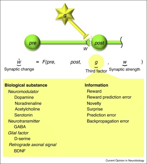
- two factor : learning based on pre- and post-synaptic neural activity.
- three factor : learning based on pre-, post-synaptic neural activity and a third factor.
Creating a learning rule in BindsNET
from bindsnet.network.nodes import Input, LIFNodes
from bindsnet.network.topology import Connection
from bindsnet.learning import PostPre

# Neurons involved in certain learning rules must record synaptic
# traces, a vector of short-term memories of the last emitted spikes.
source_layer = Input(n=100, traces=True)
target_layer = LIFNodes(n=1000, traces=True)

# Connect the two layers.
connection = Connection(
    source=source_layer, target=target_layer, update_rule=PostPre, nu=(1e-4, 1e-2)
)
nu : 2-tuple pre-,post- synaptic learning rate (how quickly synapse weight change)
weight_decay
Hebbian, WeightDependentPostPre, MSTDP, MSTDPET ...etc
요약

추후?
프로젝트...?
다음 시간,,?!
개인적으로 SNN 은 biological plausible 이 중요하다고 생각함.
Biological plausible 이 기존 DNN 에 비해 차별되는 점이자 포텐을 갖는 점.
(1. 생물학적 neuron에 가까운 spiking neuron을 사용하기 때문에 에너지 효율이 좋다 (neuromorphic processor 를써야겠지만)
2. 생물학적 뇌 처럼 범용적 능력 포텐을 가지고 있다(?) )
따라서 논문 구현이든 특정 프로젝트를 하더라도 생물학적 모티브 기반으로 적용하는게 좋지 않을까....
(ex: backpropagation 대신 backpropagation 과 동등한 능력을 가지도록 STDP learning rule 수정적용하거나, 지도학습적 형태로 teacher neuron을 설정한다거나, Dropout이 생물학적 타당하지 않으면 버리거나 생물학적 모티브를 끌어와서 적용)
Uploaded by N2T