4주차 SNN code -1

SNN code

GitHub - Shikhargupta/Spiking-Neural-Network: Pure python implementation of SNN

This is the python implementation of hardware efficient spiking neural network. It includes the modified learning and prediction rules which could be realised on hardware and are enegry efficient. Aim is to develop a network which could be used for on-chip learning as well as prediction.

https://github.com/Shikhargupta/Spiking-Neural-Network

참고하면 좋은 상준님(넨고팀원) code

Neuron

import numpy as np
import random

#defining time scale
T = 50
dt = 0.125
time = np.arange(0, T+dt, dt)

#generating random spike train to be fed to neuron
S = []
for k in range(len(time)):
		a = random.randint(0,2)
		S.append(a)


#initializing membrane potential vector
Pn = np.zeros(len(time))

#defining other parameters

Pref = 0 #resting potential
Pmin = -1 #minimun potential
Pth = 25 #threshold
D = 0.25 #leakage factor
Pspike = 4 #spike potential

count = 0 #refractory counter
t_ref = 5 #refractory period
t_rest = 0

#updating membrane potential according to simplified equations
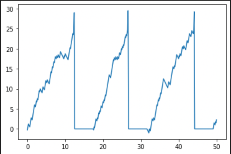
for i, t in enumerate(time):
		if i == 0:
				Pn[i] = S[i] - D
		else:
				if t<=t_rest:
						Pn[i] = Pref
				elif t>t_rest:
						if Pn[i-1]>Pmin:
								Pn[i] = Pn[i-1] + S[i] - D
						else:
								Pn[i] = 0
				if Pn[i] >= Pth:
						Pn[i] += Pspike
						t_rest = t + t_ref

membrane_potential(Pn[i]) = Pn[i-1] + input_spike(S : 0 or 1) - leakage_factor(D : 0.25)

계속 고정적인 값을 leakage 로 빼게 되는데

2가지 문제가 잇음.

1. resting potential 인 상태여도 빠지고, resting potential 보다 낮은 상태에서도 빠지게 됌.

2. 높은 potential 이든 낮은 potential이든 같은 값으로 빠지게됌.

Solution 2가지

1. 기존 LIF model 기본 식을 기준으로 computational approximation 이용.

2. 기존 LIF model 식의 analytic solution 이용. ← 이 방법은 비추천

해석적 해는 매우 powerful하지만, input이 static 하다는 가정이 있는 상태로 가정하여 풀었고, 가정은 안하게 되면 integrating form이 있어 computational 방법처럼 해결해야함.

solution 1) computational approximation

LIF neuron 기본식을 다시 보면,

$$\begin{align} \tau_{m} {du \over dt} &= -[u(t)-u_{rest}]+RI(t) \\ {du \over dt} &= - {1 \over \tau_{m}}[u(t) - u_{rest}]+{R \over \tau_{m}}I(t) \end{align}$$

이렇게 쓸수 있고, approximation 하면

$$\begin{align} \Delta u &\approx {du \over dt} \Delta t \\&=- {\Delta t \over \tau_{m}} [u(t) - u_{rest}] + {R \Delta t \over \tau_{m}} I(t) \end{align}$$

이렇게 된다. 따라서 $u(t+\Delta t) = u(t) + \Delta u$ 라고 하면,

'''
기존code
Pn[i] = Pn[i-1] + S[i] - D
'''

# tau_m == 1, R == 1
Pn[i] = Pn[i-1] - dt*(Pn[i-1]-Pref) + R*S[i]

solution 2) analytic solution

• analytic solution derivation

  

  $$\begin{align} I(t) &= I_{C} + I_{R} \\&= C {du \over dt} + {u-u_{rest} \over R} \end{align}$$

  $$RC {du \over dt} = -[u - u_{rest}]+RI(t)$$

  인데 $\tau = RC, V = u - u_{rest}$로 정리하면 $\tau {dV \over dt} = -V + RI(t) \quad … (1)$

  여기서

  i. homogeneous solution

  $I(t) = 0$, homogeneous solution 을 구해보면(1) 식이 $\tau {dV  \over dt} =  -V$ 가 되어서, $V_p = Ae^{t \over \tau}$

  ii. nonhomogeneous solution

  $I(t) \neq 0$, nonhomogeneous solution 을 구해보면 $\tau {dV  \over dt} =  -V + RI(t)$에서 $\tau dV + (V-RI(t))dt = 0$ 로 쓸 수 있는데 exact 하지 않으므로 integrating factor $F(t)$ 를 곱하여 exact 하게 만들어보면

  $$F(t) \tau dV + F(t) (V-RI(t))dt = 0$$

  Exact 한다면

  $${\partial \over \partial t} ( F(t) \tau) = {\partial \over \partial V} (F(t) (V-RI(t))$$

  이 식을 만족해야하므로 $\tau F’(t)  = F(t)$ 을 만족하는 F(t)중에 $F(t) = e^{t \over \tau}$ 를 고를 수 있다.

  다시 (1) 식으로 돌아와서 $F(t)$를 곱하면

  $$\begin{align} \tau e^{t \over \tau} {dV \over dt} + e^{t \over \tau} V &= e^{t \over \tau} R I(t) \\ {d \over dt} (\tau e^{t \over \tau} V) &= e^{t \over \tau} R I(t) \quad \\ \int_{-\infty}^t {d \over dt'} (\tau e^{t' \over \tau} V) dt'&= \int_{-\infty}^t e^{{t’ \over \tau}} R I(t’) dt’ \quad \\ \tau e^{t \over \tau} V &= \int_{-\infty}^t e^{{t’ \over \tau}} R I(t’) dt’ \quad \end{align}$$

  따라서 nonhomogeneous solution $V_{h}$은

  $$V_{h} = {1 \over C} \int_{-\infty}^t  e^{-{(t-t’) \over \tau}}  I(t’) dt’$$

  i) ,ii) 에서 구한 solution 합이 식 (1) 의 최종 solution이 되므로

  $$\begin{align} V &= V_{p} + V_{h} \\ &= Ae^{t \over \tau} + {1 \over C} \int_{-\infty}^t e^{-{(t-t’) \over \tau}} I(t’) dt’ \quad \end{align}$$

  이제 $I(t)$ 의 상황을 가정해보자.

  $$I(t) = \begin{cases} 0 \quad\quad  if\,\, t \le 0 \\  I_{0} \quad\quad  if \,\, t>0 \end{cases}$$

  (2)식에 $I(t)$ 를 대입하면,

  $$\begin{align} V &= Ae^{t \over \tau} + {1 \over C} \int_{0}^t e^{-{(t-t’) \over \tau}} I_{0} dt’ \\ &= Ae^{t \over \tau} + {I_{0} \over C} [ \tau e^{-{(t-t’) \over \tau}} ]^{t’=t}_{t’=0} \\ & = Ae^{t \over \tau} + {I_{0} \tau \over C}(1- e^{-{t \over \tau}}) \\ &= Ae^{t \over \tau} + {I_{0} R}(1- e^{-{t \over \tau}}) \end{align}$$

  여기서 boundary condition 으로 $V(0) = V_{0}$ 를 넣으면 $A = V_{0}$ 이 된다.

  최종식은

  $$\begin{align} V & = V_{0}e^{t \over \tau} + {I_{0} R}(1- e^{-{t \over \tau}}) \\ &= V_{0} + {(I_{0} R- V_{0})}(1- e^{-{t \over \tau}}) \quad \end{align}$$

# update voltage using discretized lowpass filter
# since v(t) = v(0) + (J - v(0))*(1 - exp(-t/tau)) assuming
# J is constant over the interval [t, t + dt)
voltage -= (J - voltage) * np.expm1(-delta_t / self.tau_rc)

analytic solution을 활용하려면 code 를 수정해서 적용해야함.

(위 code 는 nengo framework의 source code를 가지고옴)

Synpase

synapse : n x m # Weight (transpose)

S_in : m x len(time) #spike_in

import numpy as np
import random
from matplotlib import pyplot as plt

#constant global parameters which are same for the whole network
global Pref, Pmin, Pth, D, Pspike, time, T, dt
T = 500
dt = 0.125
Pref = 0
Pmin = -1
Pth = 5
D = 1
Pspike = 4
t_ref = 5
time  = np.arange(0, T+dt, dt)

#neuron class which can be instantiated in the main function as many times as required. It follows the integrate and fire model. 
#The out function takes in the matrices of spikes and weights and returns the output train of spikes.
class Neuron:
		def __init__(self):
				self.t_rest = 0
				self.Pn = np.zeros(len(time))
				self.spike = np.zeros(len(time))
		def out(self,S, w):
				for i, t in enumerate(time):
						if i==0:
								a1 = S[:,i]
								self.Pn[i] = np.dot(w,a1) - D
								self.spike[i] = 0
						else:
								if t<=self.t_rest:
										self.Pn[i] = Pref
										self.spike[i] = 0
								elif t>self.t_rest:
										if self.Pn[i-1]>Pmin:
												a1 = S[:,i]
												self.Pn[i] = self.Pn[i-1] + np.dot(w,a1) - 0.25 #0.25 -> D
												self.spike[i] = 0
										else:
												self.Pn[i] = 0
												self.spike[i] = 0	
								if self.Pn[i]>=Pth:
									self.Pn[i] += Pspike
									self.t_rest = t + t_ref
									self.spike[i] = 1
			
				return self.spike			
	

if __name__=='__main__':
		m = 5 #Number of neurons in first layer
		n = 3 #Number of neurons in second layer
    #creating two layers of m and n neurons
		layer1 = []
		layer2 = []
	
		for i in range(m):
				a = Neuron()
				layer1.append(a)
		for i in range(n):
				a = Neuron()
				layer2.append(a)	
	
	#initialising synapse array with random integers
		synapse = np.random.randint(0, 5, size=(n,m))
		S_in = []
	
	#initialising the input spike trains
		for l in range(m):
				temp = []
				for k in range(len(time)):
						a = random.randrange(0,2)
						temp.append(a)
				S_in.append(temp)
	
	#output of the first layer
		out_l1 = []
		w_in = np.eye(m)
		S_in = np.array(S_in)
		for l in range(m):
				temp = []
				temp = layer1[l].out(S_in,w_in[l])
				out_l1.append(temp)
		out_l1 = np.array(out_l1)	
		
	#output of the second layer which was fed with the output of the first layer
		out_l2 = []
		for l in range(n):
				temp  = []
				temp = layer2[l].out(out_l1,synapse[l])
				out_l2.append(temp)

Receptive field

convolution filter

import numpy as np
import random

#Initializing a random input matrix. During implementation this would be a 16x16 image
inp = np.random.randint(0, 255, size=(16,16)) #255? 256?

w = np.zeros([5,5]) #5x5 window initialized with zeros
pot = np.zeros([16,16]) #Initializing membrane potential matrix for 256 input neurons 
ran = [-2,-1,0,1,2] #Weight vectors for the window
ox = 2 #Origin x coordinate in the window matrix
oy = 2 #Origin y coordinate in the window matrix
w[ox][oy] = 1 #Manhattan distance zero

#Assigning weights to matrix elements according to mahanttan distance from the origin 
for i in range(5):
		for j in range(5):
				d = abs(ox-i) + abs(oy-j)
				w[i][j] = (-0.375)*d + 1

#Calculating membrane potential for each of the 256 input neurons		
for i in range(16):
		for j in range(16):
				summ = 0
				for m in ran:
						for n in ran:
								if (i+m)>=0 and (i+m)<=15 and (j+n)>=0 and (j+n)<=15: #zero padding
										summ = summ + w[ox+m][oy+n]*inp[i+m][j+n] # convolution 
				pot[i][j] = summ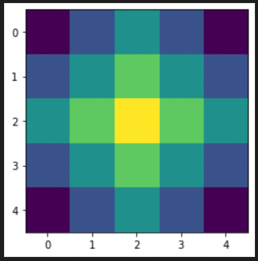

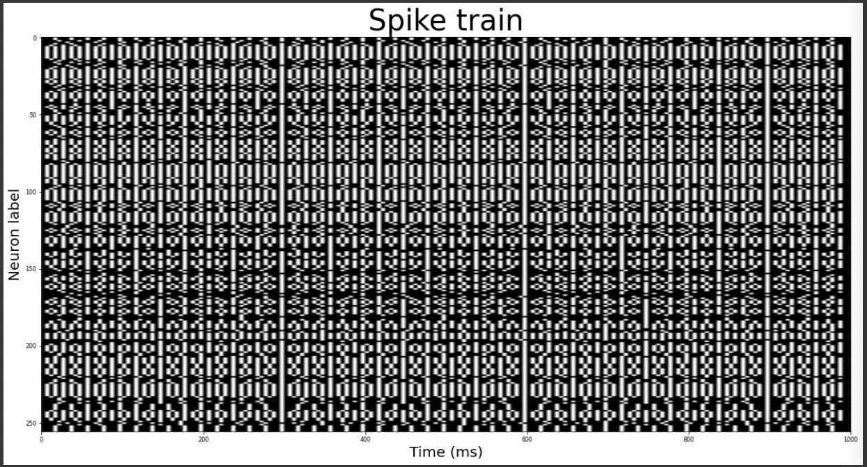
Spike train

import numpy as np
import cv2
import math
from matplotlib import pyplot as plt

# Sliding window implementation of receptive field
w = np.zeros([5,5])
pot = np.zeros([16,16])
ran = [-2,-1,0,1,2]
ox = 2
oy = 2
w[ox][oy] = 1

for i in range(5):
		for j in range(5):
				d = abs(ox-i) + abs(oy-j)
				w[i][j] = (-0.375)*d + 1

#reading dataset image (16x16)
#img = cv2.imread('1.png', 0)
img = cv2.imread('/content/drive/MyDrive/flip_SNN/Spiking-Neural-Network/images/test.png', 0)


#calculating potential map of the image (256 input neuron potential)
for i in range(16):
		for j in range(16):
				summ = 0
				for m in ran:
						for n in ran:
								if (i+m)>=0 and (i+m)<=15 and (j+n)>=0 and (j+n)<=15:
										summ = summ + w[ox+m][oy+n]*img[i+m][j+n]
				pot[i][j] = summ
    
#defining time frame of 1s with steps of 5ms
T = 1;
dt = 0.005
time  = np.arange(0, T+dt, dt)

#initializing spike train
train = []

for l in range(16):
		for m in range(16):
		
				temp = np.zeros([201,])
				#calculating firing rate proportional to the membrane potential
				freq = math.ceil(0.102*pot[l][m] + 52.02)
				freq1 = math.ceil(200/freq) #ISI(InterSpike Interval -unit (frame dt) = 5ms) or Period
		
				#generating spikes according to the firing rate
				k = 0
				while k<200:
						temp[k] = 1
						k = k + freq1
				train.append(temp)

Uploaded by N2T